R で、最小二乗法を利用して、2 次近似曲線などの高次近似曲線を描く場合は、nls 関数を利用する。nls 関数を利用するとき、データの他に、近似させたい関数の数式および初期値を入力として与える。

2 次近似曲線

x <- runif(100)
y <- 10 * x ^2 + 10 + rnorm(100)

plot(x, y, xlim = range(x), ylim = range(y))

f <- y ~ a*x^2 + b*x + c
obj <- nls(f, start = c(a = 0, b = 0, c = 0))
obj
## Nonlinear regression model
##   model: y ~ a * x^2 + b * x + c
##    data: parent.frame()
##      a      b      c
## 11.558 -2.007 10.352
##  residual sum-of-squares: 129.7
## Number of iterations to convergence: 1
## Achieved convergence tolerance: 2.564e-08

df <- data.frame(x = seq(0, 10, length = 1000))
yy <- predict(obj, df)

par(new = T)
plot(df$x, yy, type = "l", col = "darkred", lwd = 2,
     xlim = range(x), ylim = range(y), xlab = "", ylab = "")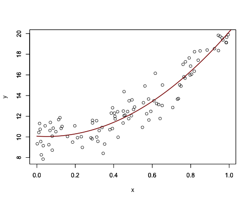

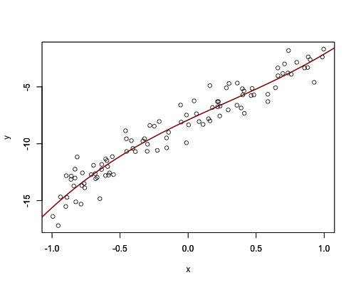
3 次近似曲線

x <- runif(100, -1, 1)
y <- 2 * x ^ 3 - x ^ 2 + 5 * x - 10 + rnorm(100, 2, 1)
plot(x, y, xlim = range(x), ylim = range(y))

f <-  y ~ a*x^3 + b*x^2 + c*x + d
obj <- nls(f, start = c(a = 0, b = 0, c = 0, d = 0))
obj
## Nonlinear regression model
##   model: y ~ a * x^3 + b * x^2 + c * x + d
##    data: parent.frame()
##       a       b       c       d
##  1.1161 -0.9615  5.6329 -7.9046
##  residual sum-of-squares: 100.1
## Number of iterations to convergence: 1
## Achieved convergence tolerance: 2.96e-08

df <- data.frame(x = seq(-10, 20, length = 1000))
yy <- predict(obj, df)
 
par(new = T)
plot(df$x, yy, type = "l", col = "darkred", lwd = 2,
     xlim = range(x), ylim = range(y), xlab = "", ylab = "")