Python で LASSO 回帰を行うためのサンプルデータを作成する。真の説明変数として 2 つ(z1, z2)を作り、真の説明変数にノイズを与えて 5 つの説明変数(x1, x2, x3, x4, x5)を作る。また、応答変数 y を 2z1 - z2 にノイズを加えた値とする。
import numpy as np
import pandas as pd

np.random.seed(2019)

z1 = np.random.rand(100) * 10
z2 = np.random.rand(100) * 10

x1 = z1 + np.random.normal(0, 1, 100)
x2 = z1 + np.random.normal(0, 1, 100)
x3 = 2 * z1 + np.random.normal(0, 1, 100)
x4 = z2 + np.random.normal(0, 1, 100)
x5 = -3 * z2 + np.random.normal(0, 1, 100)


X = pd.DataFrame([x1, x2, x3, x4, x5]).T
Y = 2 * z1 - z2 + np.random.normal(0, 1, 100)
LASSO 回帰
scikit-learn パッケージの linear_model クラスで LASSO 回帰を行う Lasso メソッドが用意されている。このメソッドを使用して LASSO 回帰を行ってみる。LASSO 回帰を行うとき、正則化項の寄与の大きさを調整する正則化パラメーターをあらかじめ与える必要がある。このパラメーターを alpha 引数で指定する。まず、ここでは、仮に正則化パラメーターとして alpha = 0.1 と指定して回帰を行ってみる。
from sklearn.preprocessing import StandardScaler
from sklearn.linear_model import Lasso

scaler = StandardScaler()
clf = Lasso(alpha=0.1)

scaler.fit(X)
clf.fit(scaler.transform(X), Y)
## Lasso(alpha=0.1, copy_X=True, fit_intercept=True, max_iter=1000,
##    normalize=False, positive=False, precompute=False, random_state=None,
##    selection='cyclic', tol=0.0001, warm_start=False)

print(clf.coef_)
## [ 0.46288203  1.05025169  3.86729005 -0.84086274  2.24241141]

print(clf.intercept_)
## 5.666182032044889
クロスバリデーション
最適な正則化パラメーターを決めるためにはクロスバリデーションを行う必要がある。scikit-learn パッケージの linear_model クラスにはクロスバリデーションと LASSO 回帰を同時に実行してくれる LassoCV メソッドが用意されている。ここで、最適な λ を 5-fold クロスバリデーションにより、10-6 ≤ α ≤ 102 の範囲内で 0.1 間隔のグリッドサーチを行なって決定する例を示す。
from sklearn.preprocessing import StandardScaler
from sklearn.linear_model import LassoCV

scaler = StandardScaler()
clf = LassoCV(alphas=10 ** np.arange(-6, 1, 0.1), cv=5)

scaler.fit(X)
clf.fit(scaler.transform(X), Y)
## LassoCV(alphas=array([1.00000e-06, 1.25893e-06, ..., 6.30957e+00, 7.94328e+00]),
##     copy_X=True, cv=5, eps=0.001, fit_intercept=True, max_iter=1000,
##     n_alphas=100, n_jobs=None, normalize=False, positive=False,
##     precompute='auto', random_state=None, selection='cyclic', tol=0.0001,
##     verbose=False)

print(clf.alpha_)
## 0.005011872336272571

print(clf.coef_)
## [ 0.48686631  1.07953324  3.9316769  -0.92341824  2.27543548]

print(clf.intercept_)
## 5.666182032044889
このように、クロスバリデーションにより決定された α は 0.005 であることがわかる。また、最適な α で作られたモデルの係数および定数項は上記のように求まる。
モデル評価
モデルの作成からモデルの評価まで一通り実行する例を以下に示す。ここで、データセットの 8 割を教師データとして、LASSO 回帰を行う。このとき、最適な α を 5-fold クロスバリデーション決める。次に、教師データを除いた 2 割のデータを検証データとして LASSO モデルを検証することにする。
from sklearn.preprocessing import StandardScaler
from sklearn.linear_model import LassoCV
from sklearn.metrics import mean_squared_error
x_train, x_test, y_train, y_test = train_test_split(X, Y, test_size=0.2, random_state=0)
scaler = StandardScaler()
clf = LassoCV(alphas=10 ** np.arange(-6, 1, 0.1), cv=5)
scaler.fit(x_train)
clf.fit(scaler.transform(x_train), y_train)
y_pred = clf.predict(scaler.transform(x_test))
mse = mean_squared_error(y_test, y_pred)
print(mse)
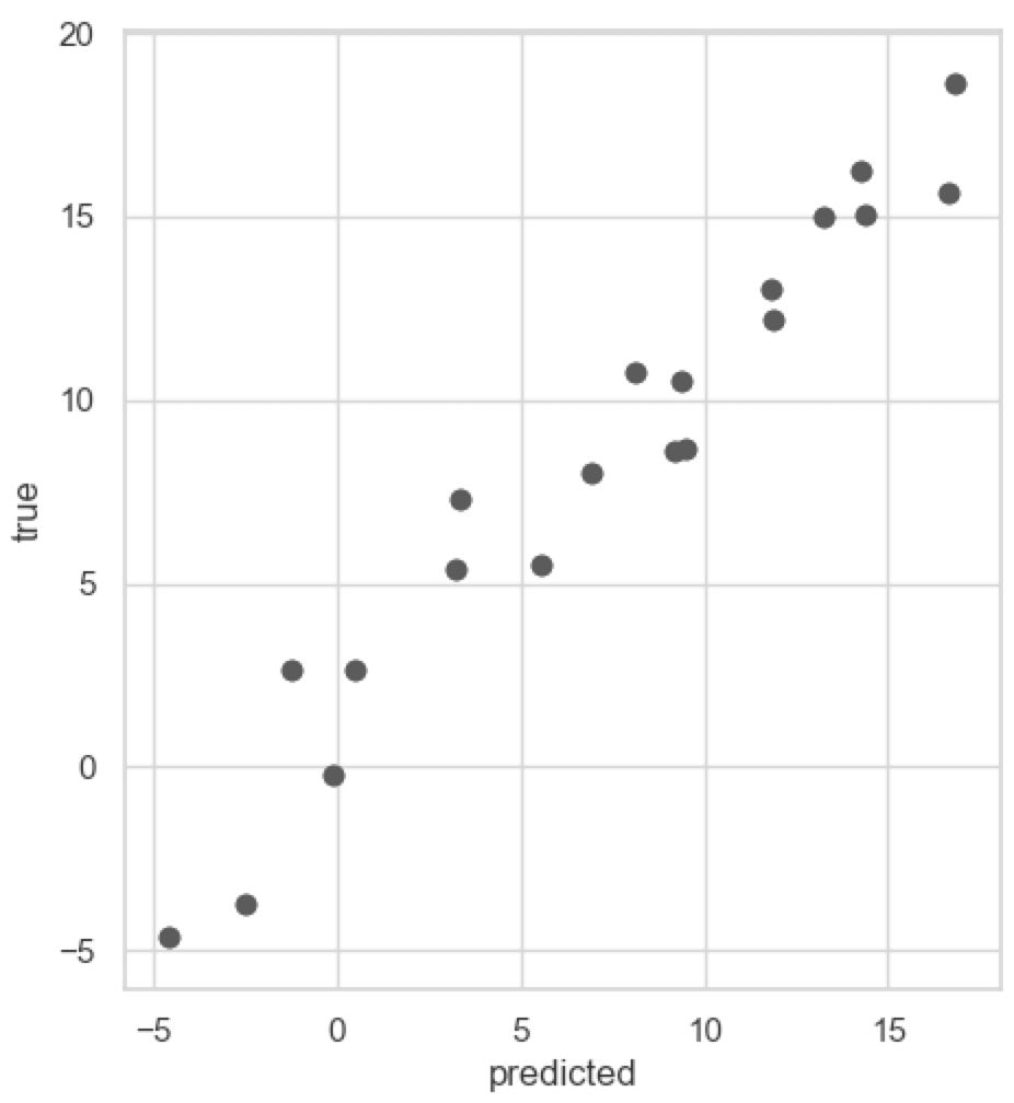
## 3.258166943313589このように、モデルの予測値と実際の観測値との平均二乗誤差が 3.258 であることが計算された。また、予測値と観測値の対応を散布図で描くとき、matplotlib パッケージを使用する。
from matplotlib import pyplot as plt
fig = plt.figure()

ax = fig.add_subplot(1, 1, 1)
ax.scatter(y_pred, y_test)
ax.set_xlabel('predicted')
ax.set_ylabel('true')
ax.set_aspect('equal')

fig.show()